Papers We Love PDX: A DNA-Based Archival Storage System
I presented a paper titled A DNA-Based Archival Storage System recently at the Papers We Love Portland meetup. I’ve always liked biology, and I’m starting to like computer science too, so I really enjoyed reading this paper. This blog post will be the bloggified version of my talk, so let’s learn something about biology and/or computer science!
The reason I like this paper is that the researchers from University of Washington and Microsoft combined two fields (biology/biochemistry and computer science) that are pretty well studied and came up with a totally new creation. At first, it might seem funny and random, but the more you think about it, the more you realize it is a super creative and immaginative way of solving a problem.
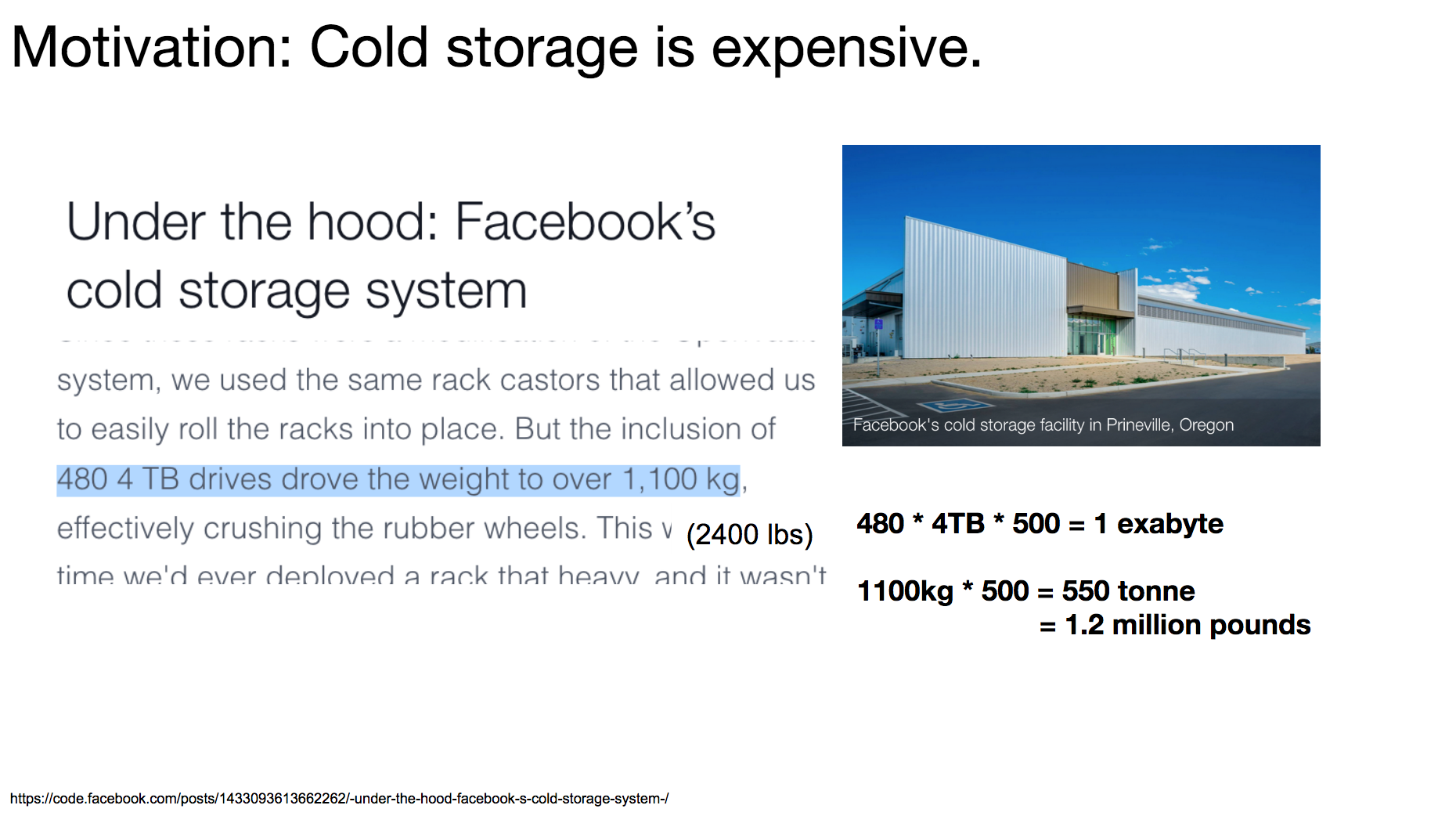
A large motivation behind this paper is that cold storage is very expensive. Cold storage is for storing some data that we need infrequently for a very long time. In 2015, Facebook built a cold storage facility that can store 1 exabyte (1 billion gigabytes). The facility contains 500 racks, each of which weighs 1,100 kg (2,400 lbs), which means just the weight of the racks is over one million pounds! Now, imagine transporting all those heavy racks, building an entire facility dedicated to it, and maintaining the facility. It is a very expensive operation for storing an exabyte.
Before we move on, I’d like to briefly introduce you to DNA (deoxyribonucleic acid). In computers, binary data is made up of bits which can either be 1 or 0. In biology, DNA is made up of nucleotides which can either be A, C, G, or T. We use the acronyms A, C, G, and T, and they stand for adanine, cytosine, guanine, and thymine.
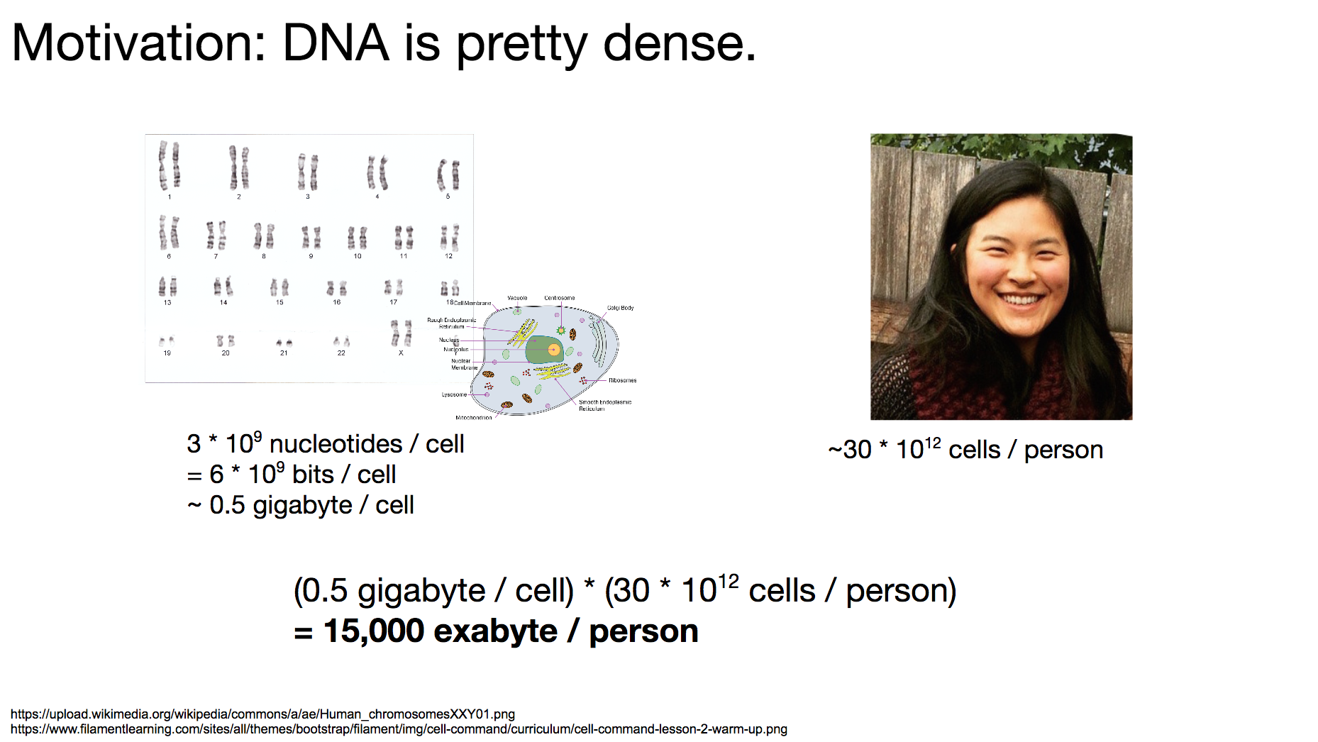
The reason researchers were interested in storing binary data in DNA is that DNA is quite dense. DNA is the language all living organisms on Earth use to store biological data. To get a sense of how dense DNA is, let’s think about how much data each person carries.
A typical single human cell contains 3 billion nucleotides, which translate to 6 billion bits worth of data. That is about a half gigabyte. Each person roughly has 30 trillion cells, which means one person carries about 15,000 exabyte of data. Compare that to Facebook’s facility for storing a single exabyte!
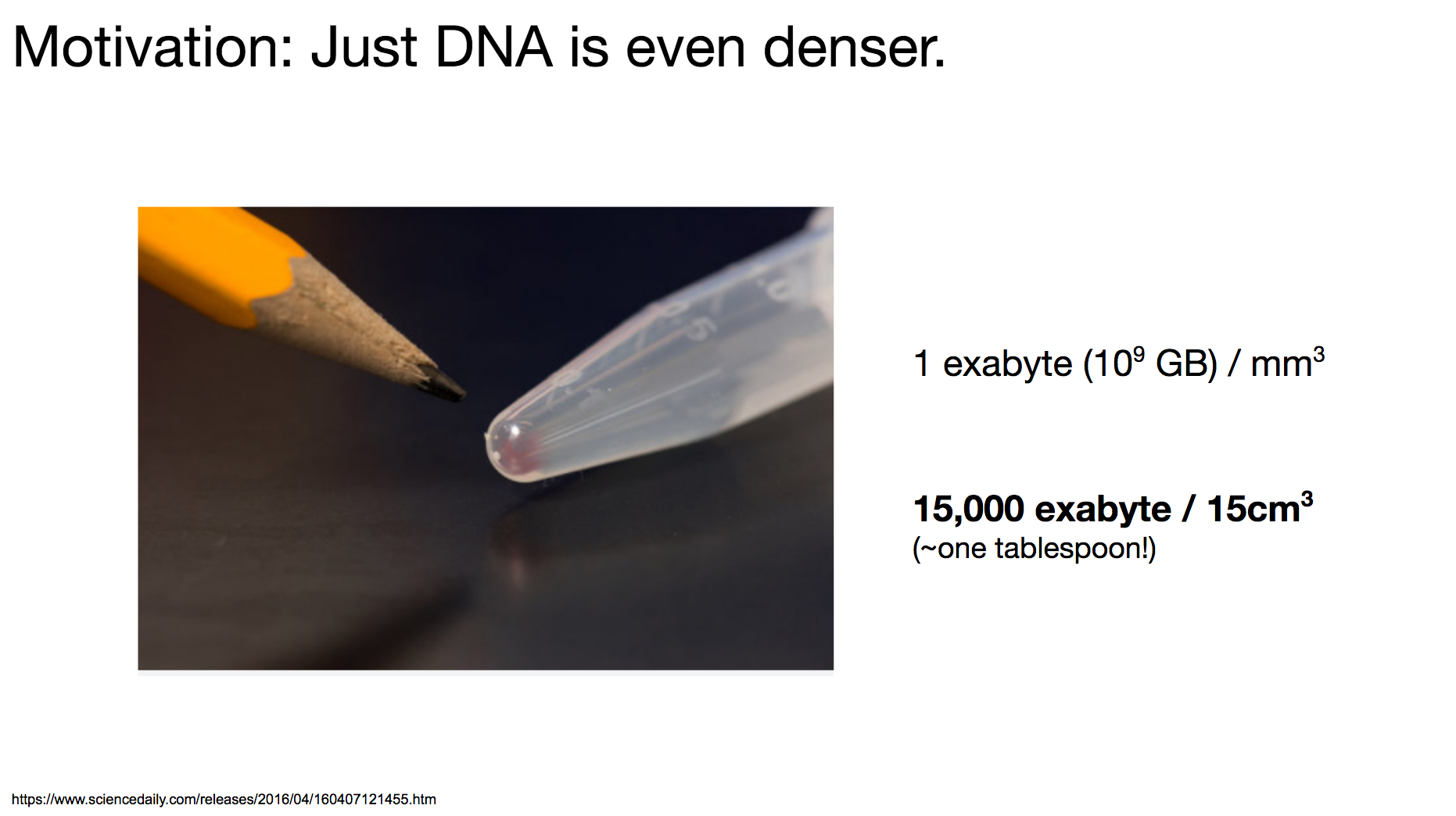
A human body is mostly non-DNA, which means when we consider just the DNA, the data density is even higher. In pure DNA, we can store an exabyte in 1 mm³, which means 15,000 exabyte can be held in a single tablespoon.
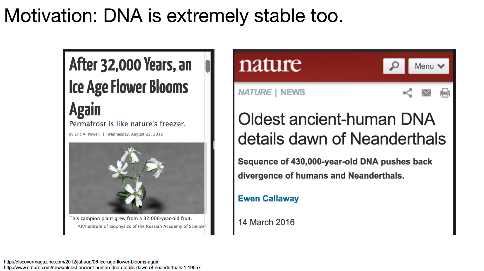
Another really huge benefit of using DNA for data storage is that DNA is extremely stable. We see on the news how people grew an ice age flower from an ice age fruit that is 32,000 years old. We see how people discovered Neanderthal DNA that is 430,000 years old, which gave us insight into the origin of humans. These DNAs were not kept in pristine condition either – they were in literal dirt and ice, and they still encoded good information that grew into a flower and bridged the gap in our knowledge.
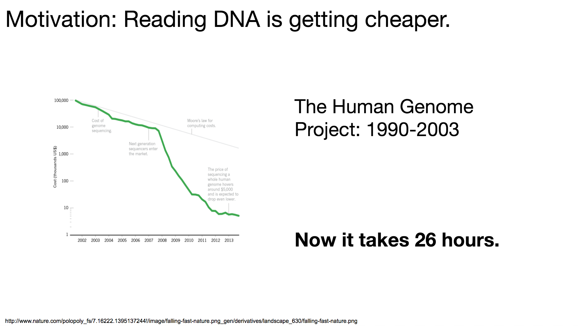
But why now? Why are the researchers starting to explore this area? It’s because reading (or sequencing) DNA is becoming cheaper and cheaper. The Human Genome Project, a collaborative project among dozens of international research institutes to read the entire human genome, launched in 1990 and took 13 years to complete. If we wanted to do the same operation (read the entire human genome) today, it can take as short as 26 hours.
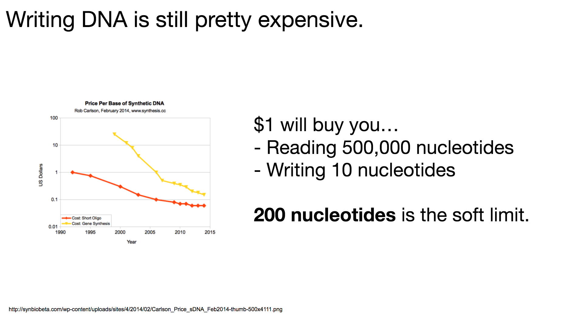
One thing to remember throughout our discussion today is that writing DNA is still pretty expensive. I believe it’s because there hasn’t been enough demand to drive the market, and it will become cheaper when more and more people become interested in synthesizing DNA. The researchers decided that 200-nucleotides-long DNA string was the most cost-effective length: long enough to encode meaningful data, but short enough to be reasonably priced.
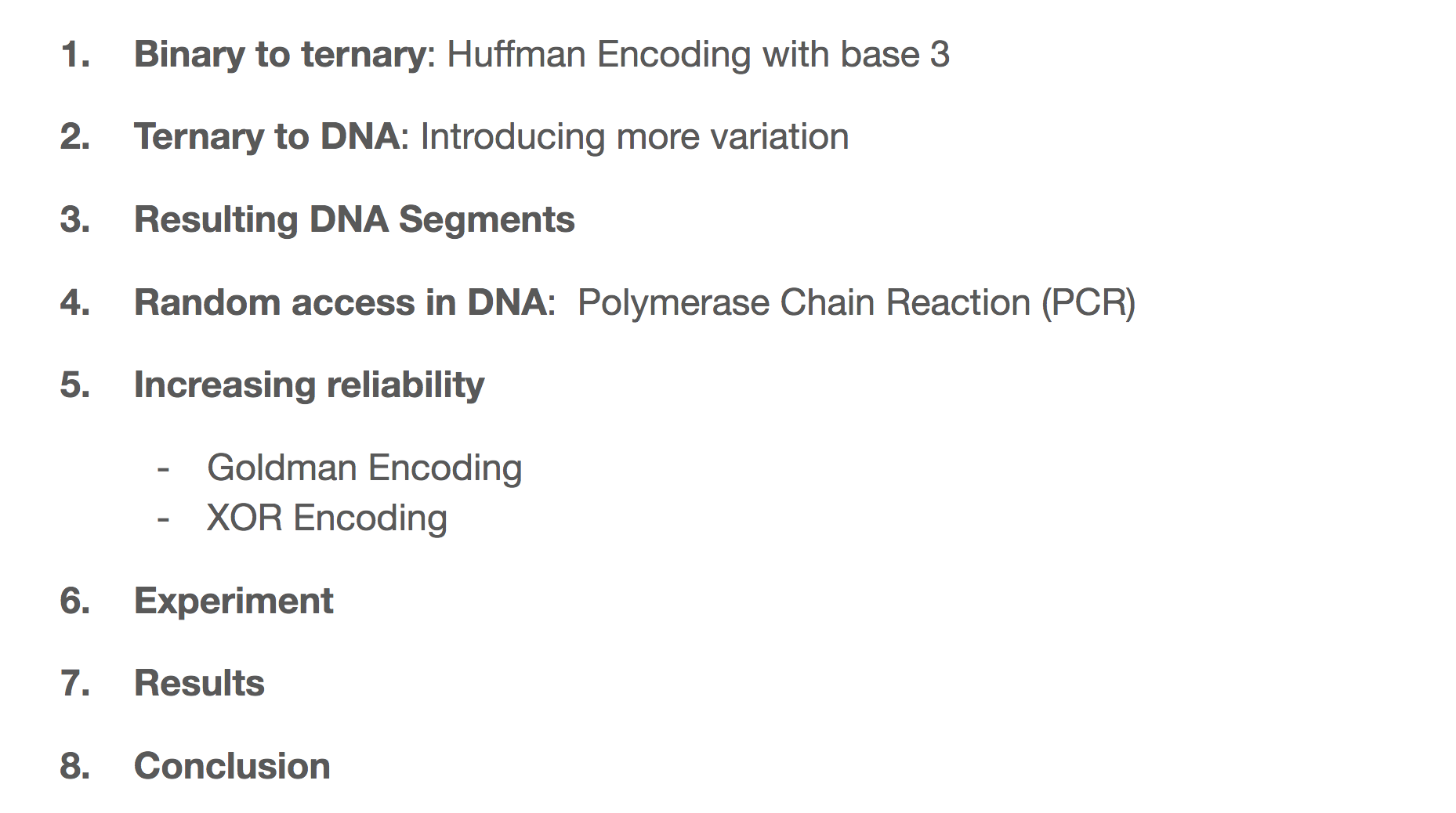
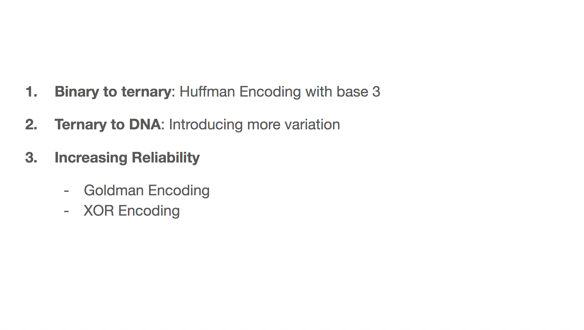
We’re going to walk through the steps the researchers took when transforming binary data into DNA. They did so in a 2-step encoding algorithm. First, they transformed binary data into ternary data through Huffman tree. Then they transformed the ternary data into DNA through a rotating table that we’ll learn soon. We’ll see what the DNA segment looks like in the end, how we can have random access to the data through PCR (Polymerase Chain Reaction). We’ll also learn how to increase reliability through two different algorithms. We’ll then learn about which files the researchers encoded and decoded, and the things they learned during the process.
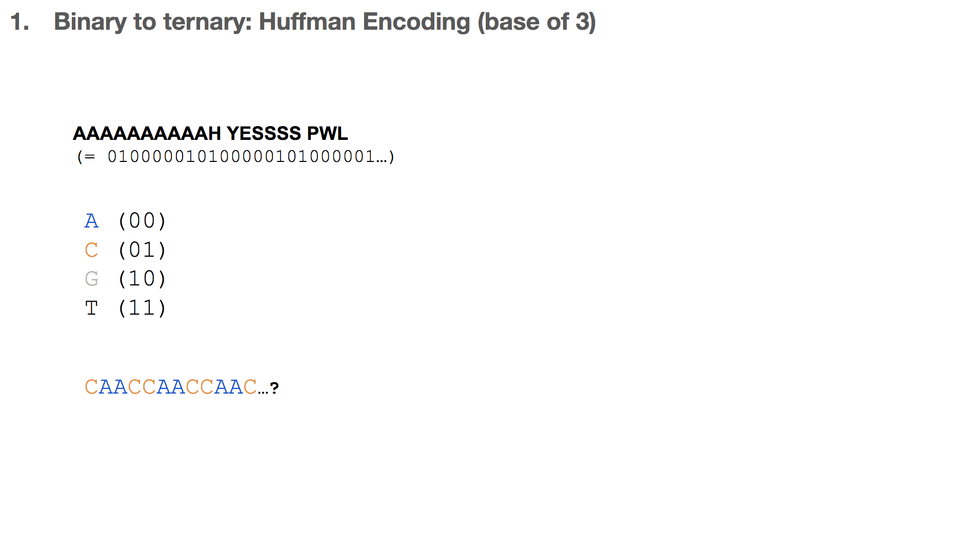
Let’s say we want to encode the sentence “AAAAAAAAAAH YESSSS PWL”, which can be represented in bits. One intuition might be assigning two bits to one nucleotide, and translating the binary data. In this case, we say that 00 is equivalent to A and so on.
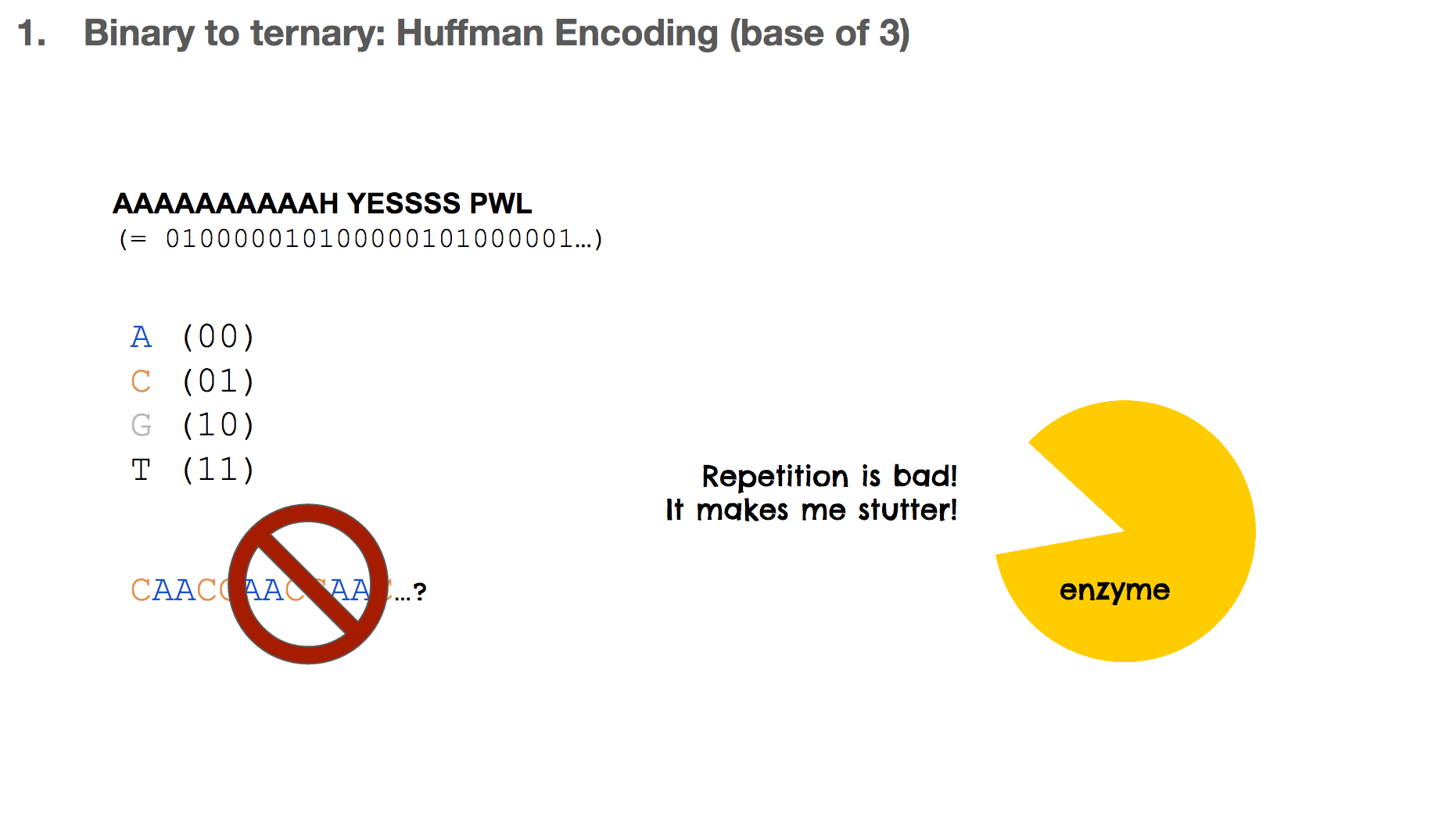
But this isn’t ideal in biochemistry, because it can result in a lot of repetitions. For example, with this scenario, “A” becomes CAAC which means ten “A”s would look like CAACCAACCAAC.... Repetition in biology/biochemistry isn’t good for two reasons: (1) enzymes, the catalysts of biochemical reactions, start to “stutter” when there is too much repetition, and (2) repetition creates homopolymers, which is “sticky” and the DNA string can bind to other DNA strings. This is like a piece of ducktape that sticks to something and becomes hard to separate.
So the researchers did a 2-step encoding algorithm, and the first step was Huffman encoding with a bast of three. Let’s see how the Huffman tree is used first. Say we have a string of encoded message, that goes 112220022.... We travel down the Huffman tree until we reach the leaf, and then we swap the path we took with the letter the path took us to. For example, 11 takes us to “T”so 11 becomes “T”. 22 takes us to “A” so 22 becomes “A”. If we keep doing that, we can decode our message, which is “TADA GO HUFFMAN”!
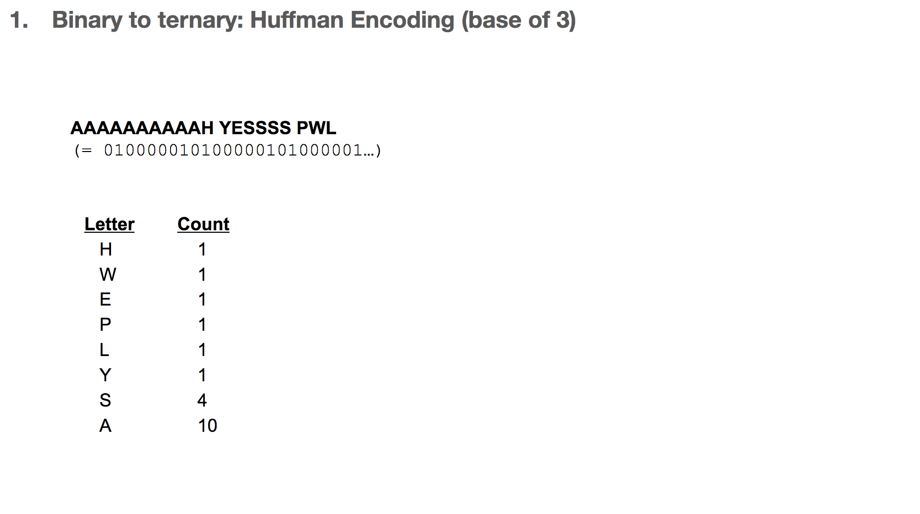
How do we build the Huffman tree? First, we record how often an element occurs in the message. For example, “H” was seen once and “A” was seen ten times.
We take the three elements with the lowest count, and group them into a single element. Its count becomes the sum of those three elements’ counts. Then we sort our list of elements, and repeat until we run out of elements to group. One group (or node) can have at most three elements, because we’re building a Huffman tree with a base of three.
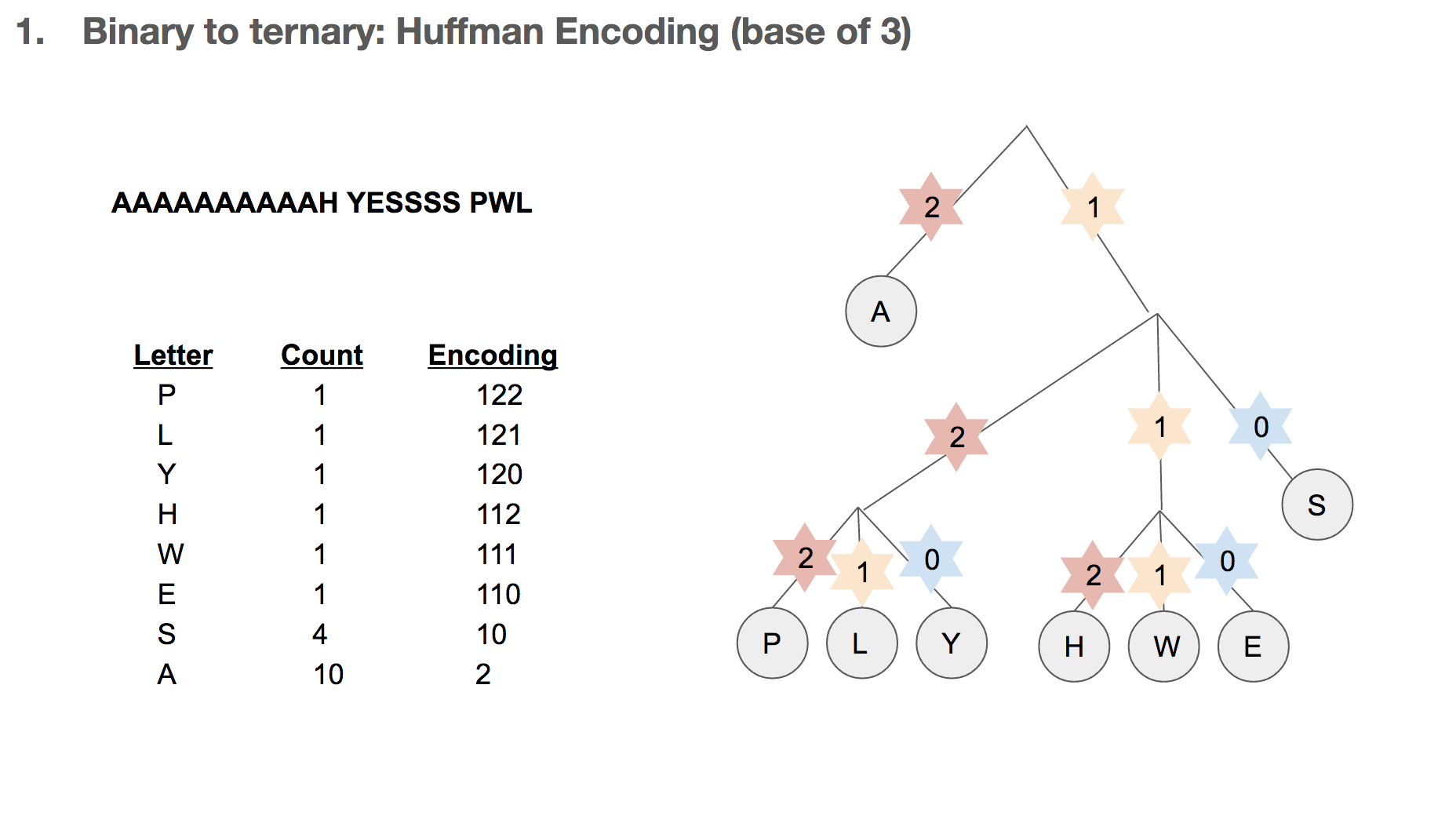
Then we record the path we take to reach a leaf (or the end of the tree). For example, in order to reach “P”, we take the path 122. In order to reach “A”, we take the path 2. Huffman coding has really interesting properties, and I highly recommend diving a little deeper!
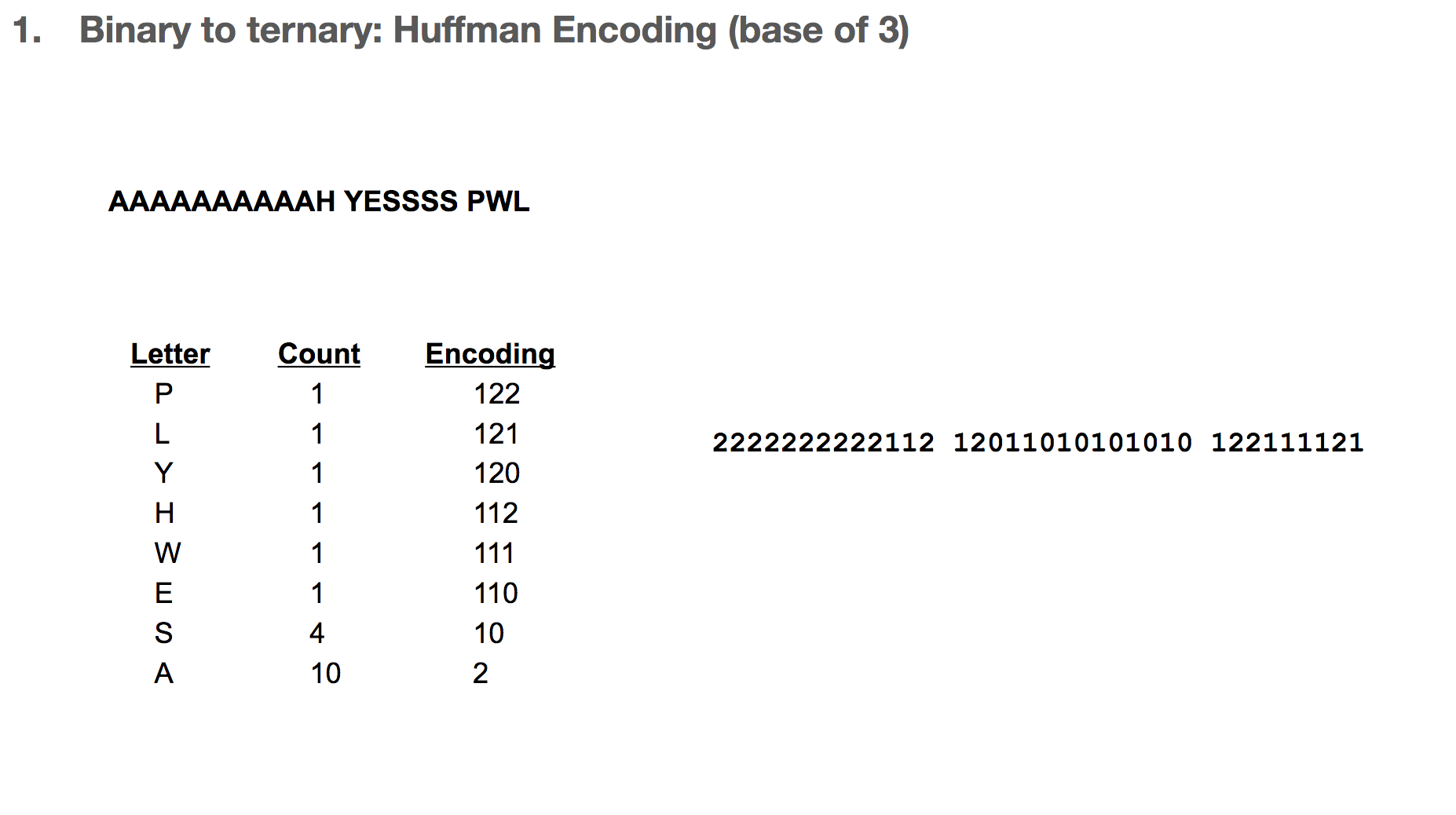
After that, we replace each letter in our message with its path in the Huffman tree. Our sentence is now encoded as 2222222222112 ....
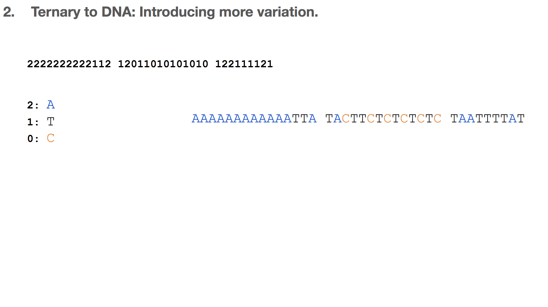
One intuition might be to assign a nucleotide to each ternery digit.
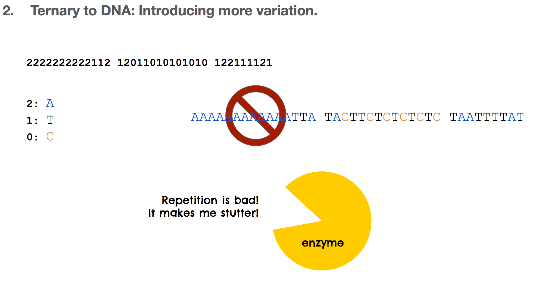
But again, this is not good for the reasons we learned earlier. Repetition makes enzymes stutter and makes DNA sticky. Not good!
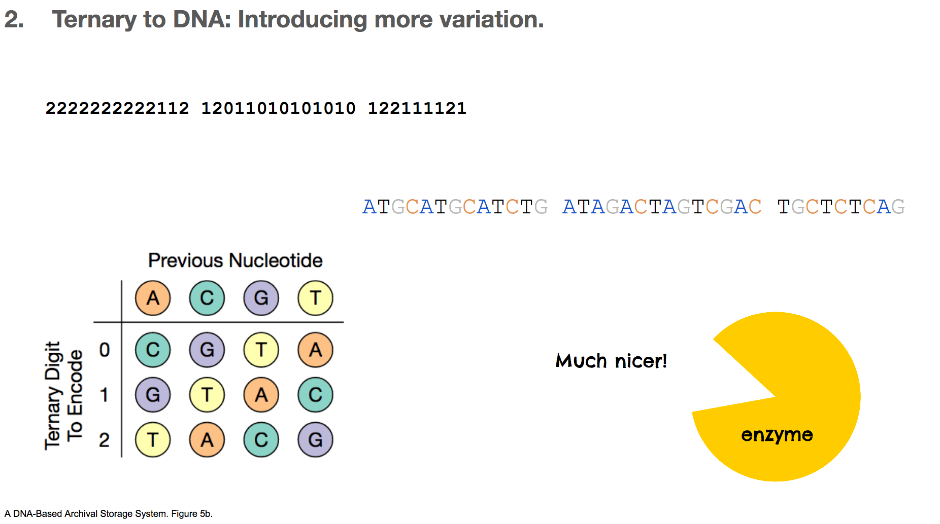
To fix this repetition issue, the researchers used a rotating table of ternary digit and nucleotide. This table decides which nucleotide will encode the current ternary digit based on the previous nucleotide. With this algorithm, there can never be two consecutive nucleotides, which alleviates the repetition problem that we’ve discussed a lot. We’ll assume that the first nucleotide is A, and our ternery digit message becomes ATGCATGC....
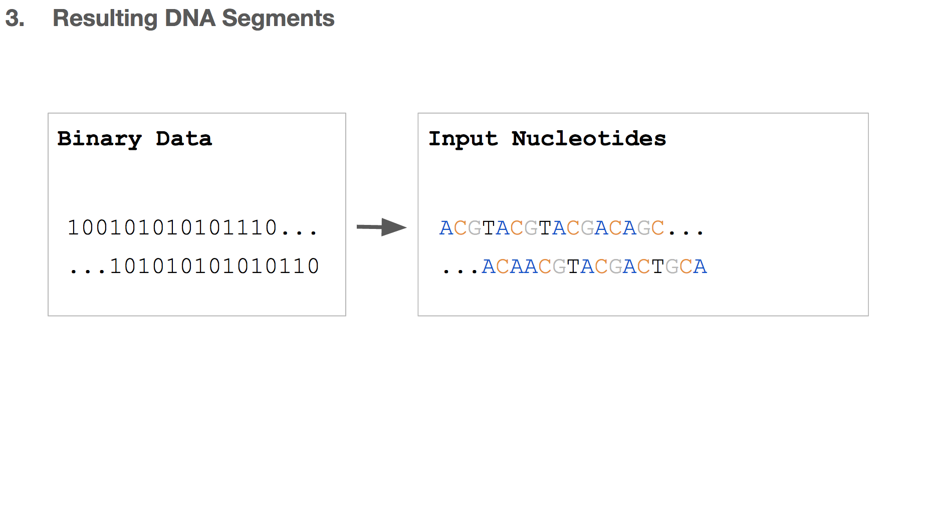
So far, we transformed some binary data into a string of DNA, which we’ll call “input nucleotides”. Input nucleotides will reflect the size of the binary data, i.e. if the original binary data is large, the input nucleotides will be long.
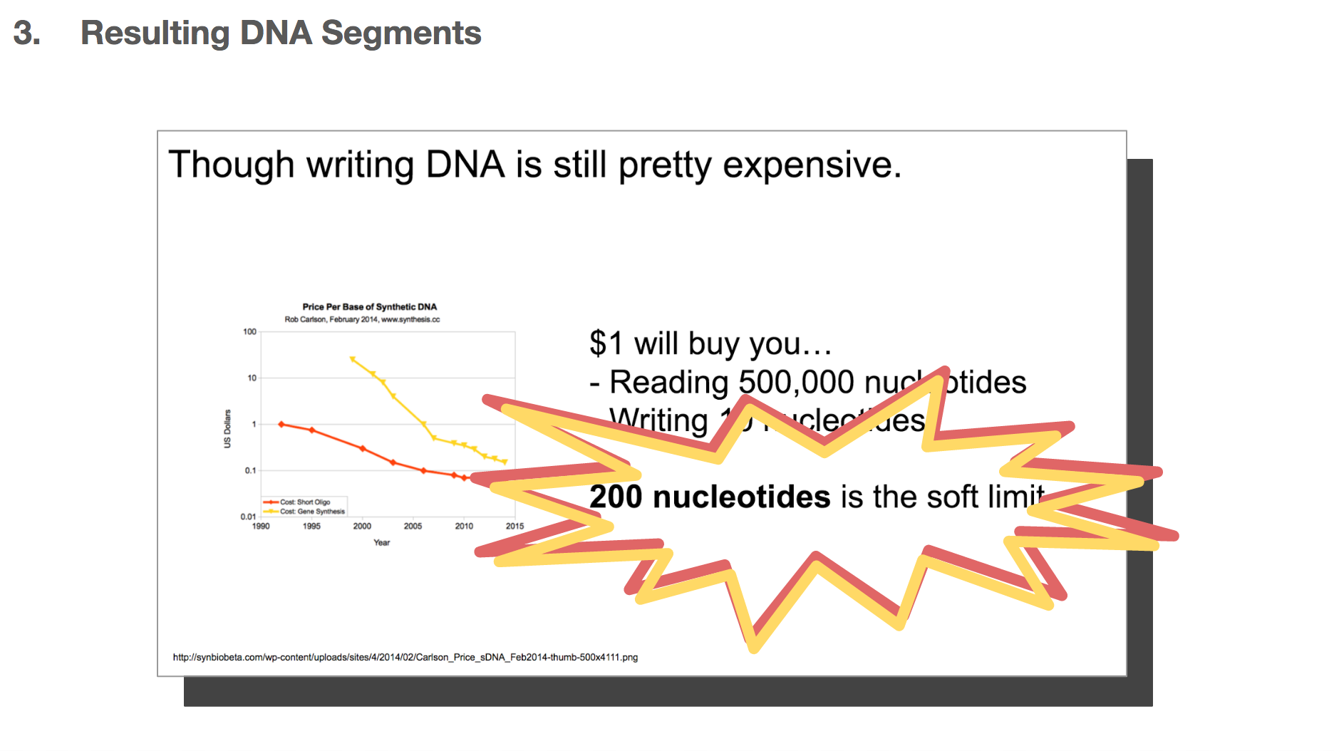
But we discussed earlier that writing DNA is expensive, and we want to limit each DNA string to be 200 nucleotides long.
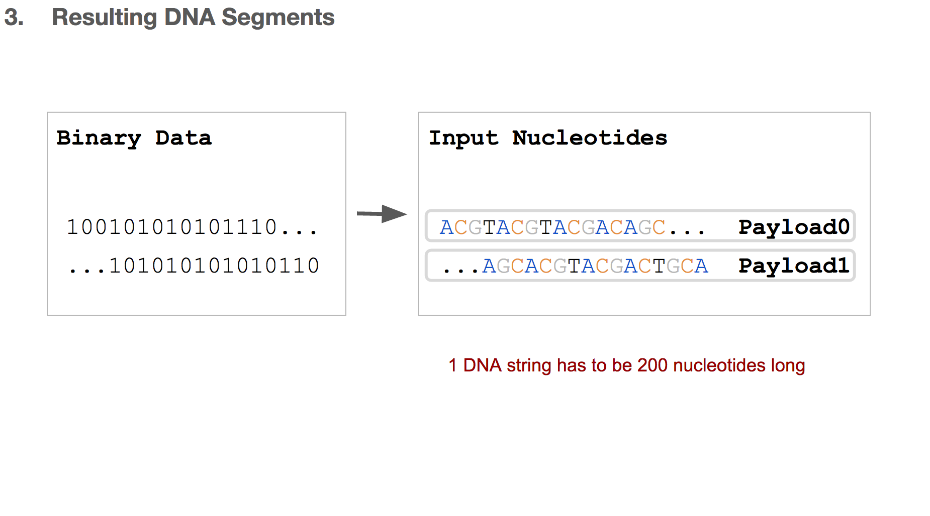
Researchers came up with a solution, which is simply breaking the input nucleotides into smaller chunks. We’ll call each chunk a “payload”.
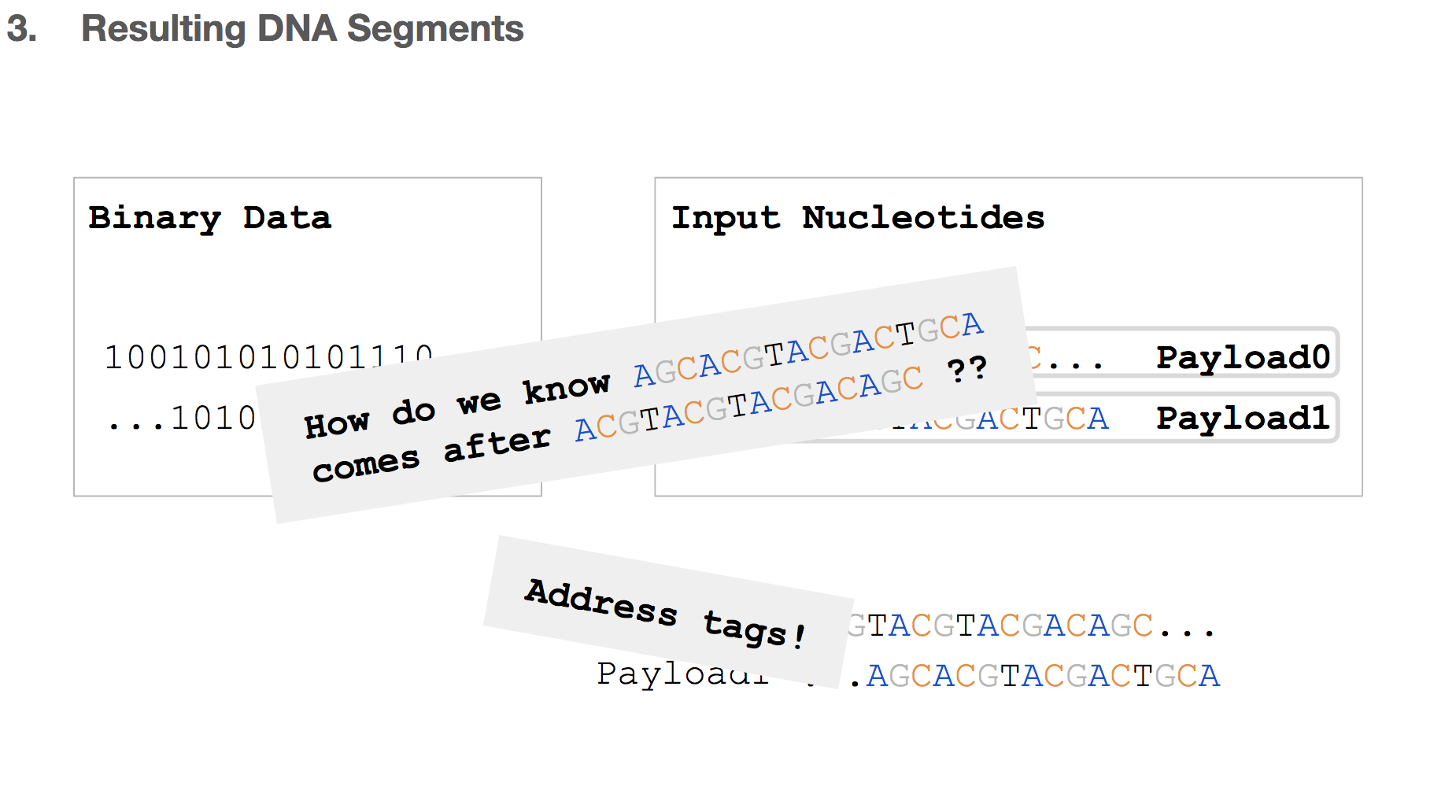
But we will be storing these DNA strings in a tube where everything will be mixed and non-ordered. So how do we know the order of these payloads? The answer to that is address tags!
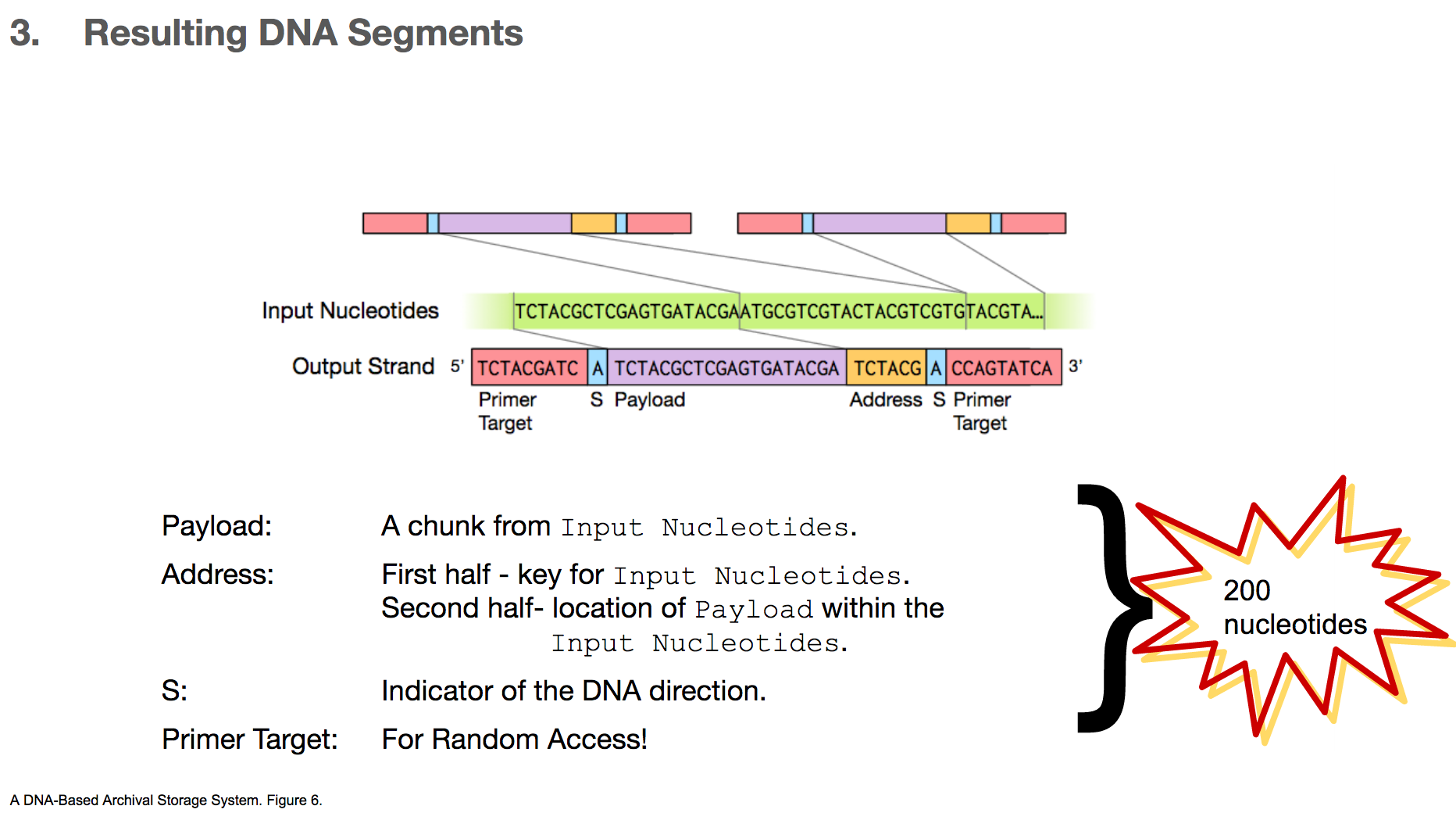
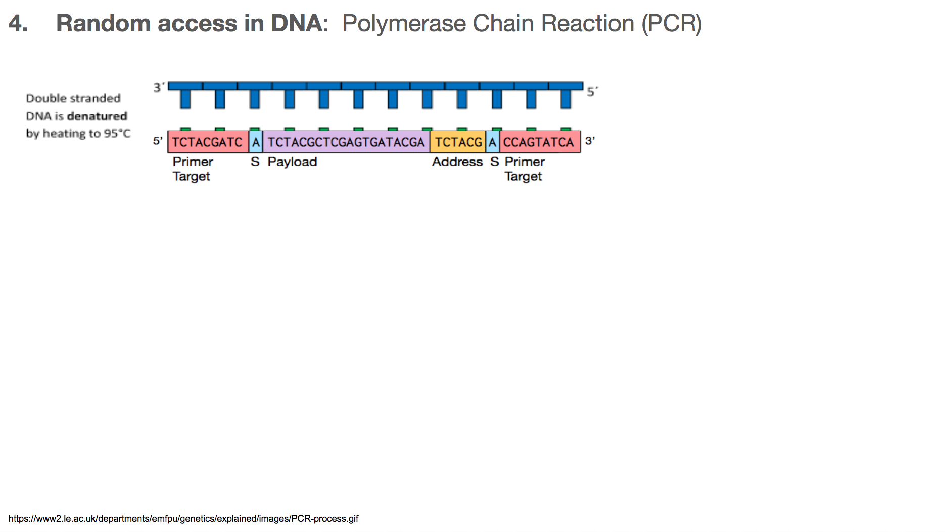
And therefore, the resulting DNA segment has many additional features.
- Payload will represent a chunk of input nucleotides.
- Address tags will come in two parts. The first part will tell us that a given payload belongs to some original file, for example “this payload is for cat.jpg”. The second part will tell us the location of this payload within the input nucleotides, for example “this payload is the first payload”.
- S shows the direction of the DNA segment, because the researchers sometimes encoded a different data in its complementary strand. We won’t go into details about this part.
- Primer target is the region a primer binds to, and this will be used for random access. We’ll talk about this in the next few slides.
All of these components will add up to 200 nucleotides.
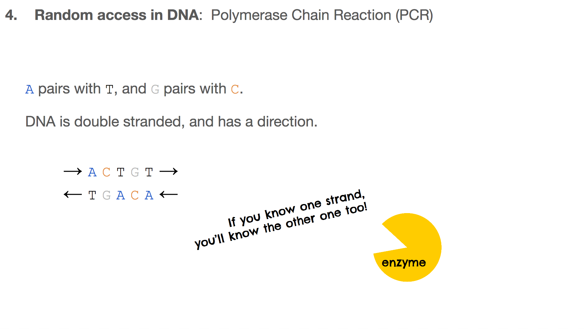
The researchers used Polymerase Chain Reaction, or PCR, for random access. In order to understand PCR, we have to remember two important features about DNA:
Abinds toTandCbinds toG.- DNA is double stranded, and they run in opposite directions.
This means that the two strands are mirror images to each other, and if you know one strand, you’ll know the other one too!
PCR is a very commonly used technology in biochemistry/biology for making lots of copies of the DNA you want using primers. Let’s walk through the steps in PCR. Say we want to amplify a DNA piece that we saw earlier in the slides. It is the bottom one in this slide. It will have a corresponding DNA strand that is the mirror image, which is the top one in this slide.
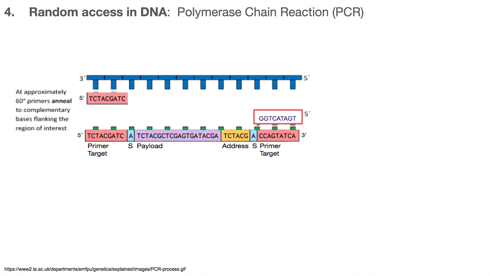
The primers will bind to primer target. Primer can be thought of as a fire starter. It is the beginning. It primes a reaction.
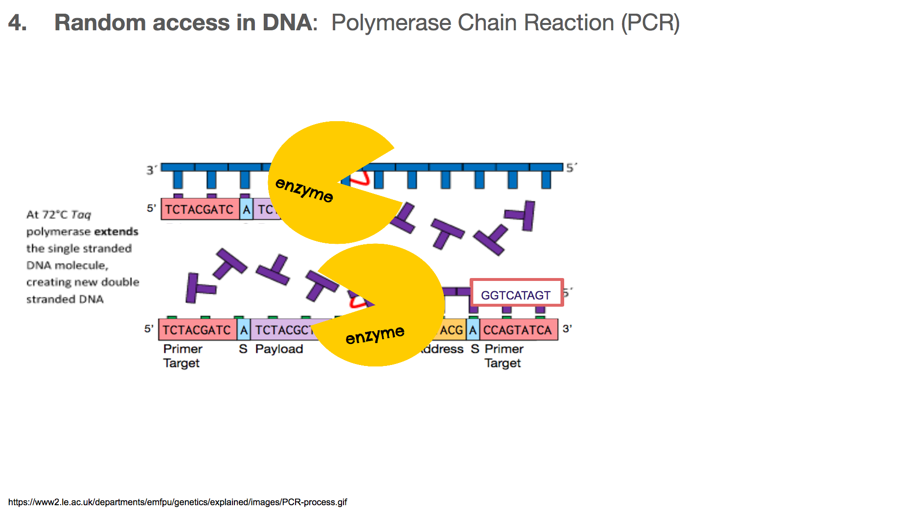
Once the primers are bound to primer targets, the enzymes know how to fill in the rest because: (1) If it sees an A in the template (or mirror image), it will fill in the blank with T. Same with C and G. (2) DNA has a direction, so the enzyme will move in one direction, meaning the enzyme-created-DNA will grow in only one direction.
At the end of a PCR, we will have two copies of the DNA we want, when we started with only one.
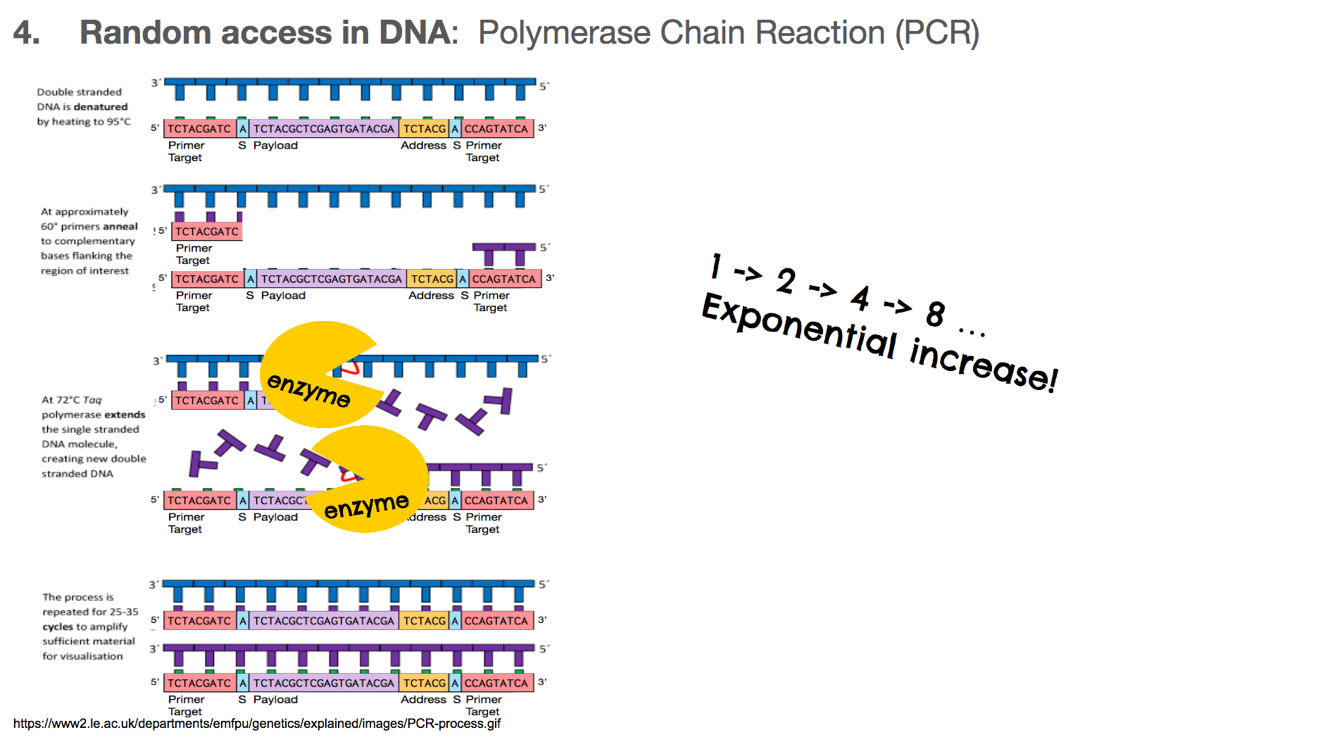
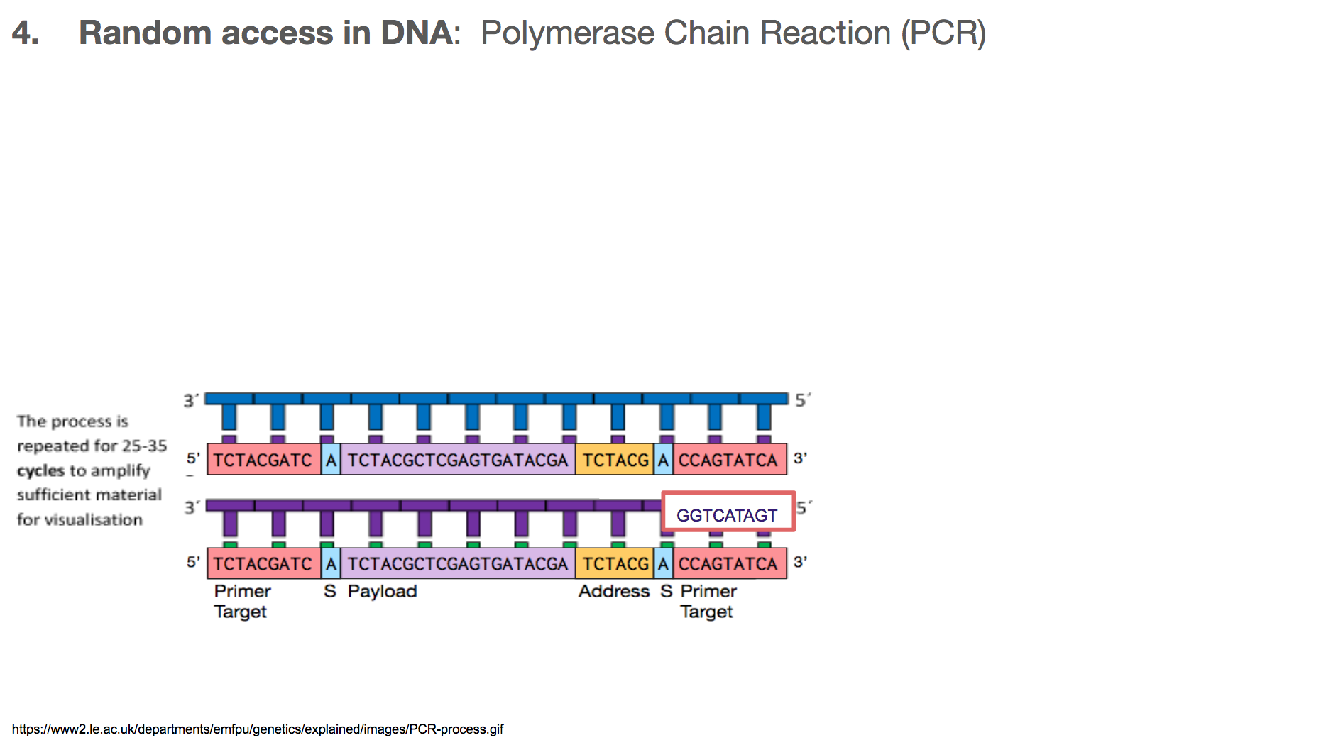
At the end of the next round of PCR, we will have 4 copies, then 8, then 16, and so on. This means that the number of DNA we want grows exponentially. Typically, a biologist runs about 30 rounds of PCR, meaning at the end of the entire reaction, there will be over one billion copies of the DNA we want!
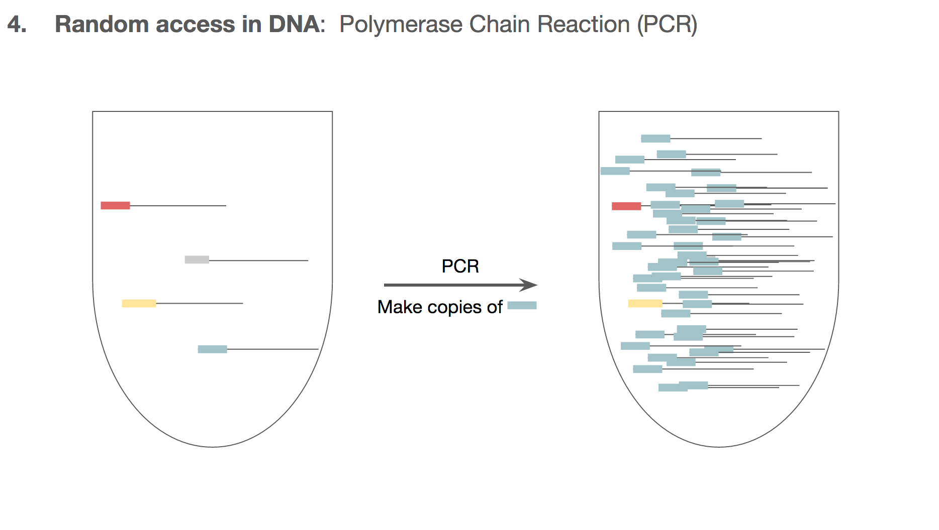
PCR doesn’t make the unwanted DNA strings go away. But by the end of PCR, the number of the DNA we want will outnumber the unwanted DNA by such a large magnitude that the unwanted DNA becomes almost like a noise in data. And this is how the researchers established random access in the DNA encoded data.
We can make sure all the cat.jpg related DNA strings to have the same primer target. This means that if we want to retrieve cat.jpg from a tube of all kinds of mixed DNA strings, we will specifically amplify only the cat.jpg related DNA strings using the primers. We won’t have to go through a catalogued list of DNA strings, and we can access just the file we want through primers.
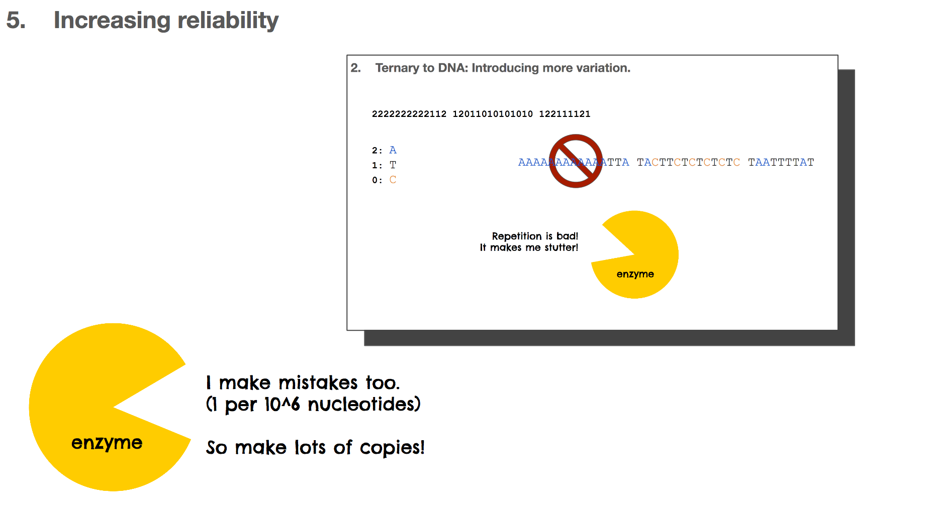
Throughout this presentation, we learned many times that enzymes make mistakes. These mistakes are often beneficial because it gives life to try out new paths which is one method of evolution. But these mistakes are not great for the DNA based storage system because it means that the data can be altered when they shouldn’t. One way to overcome this is by making lots of copies so that when a copy becomes altered, there will be other correct copies to rescue the mistake.
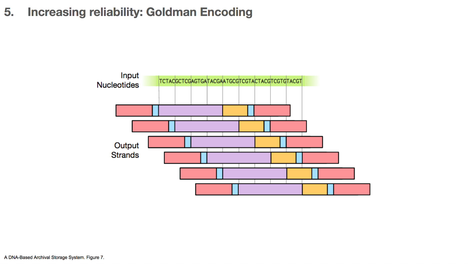
One algorithm the researchers used for increasing reliability is Goldman encoding. This algorithm uses a “sliding window” to take a view into the input nucleotides and create a payload.
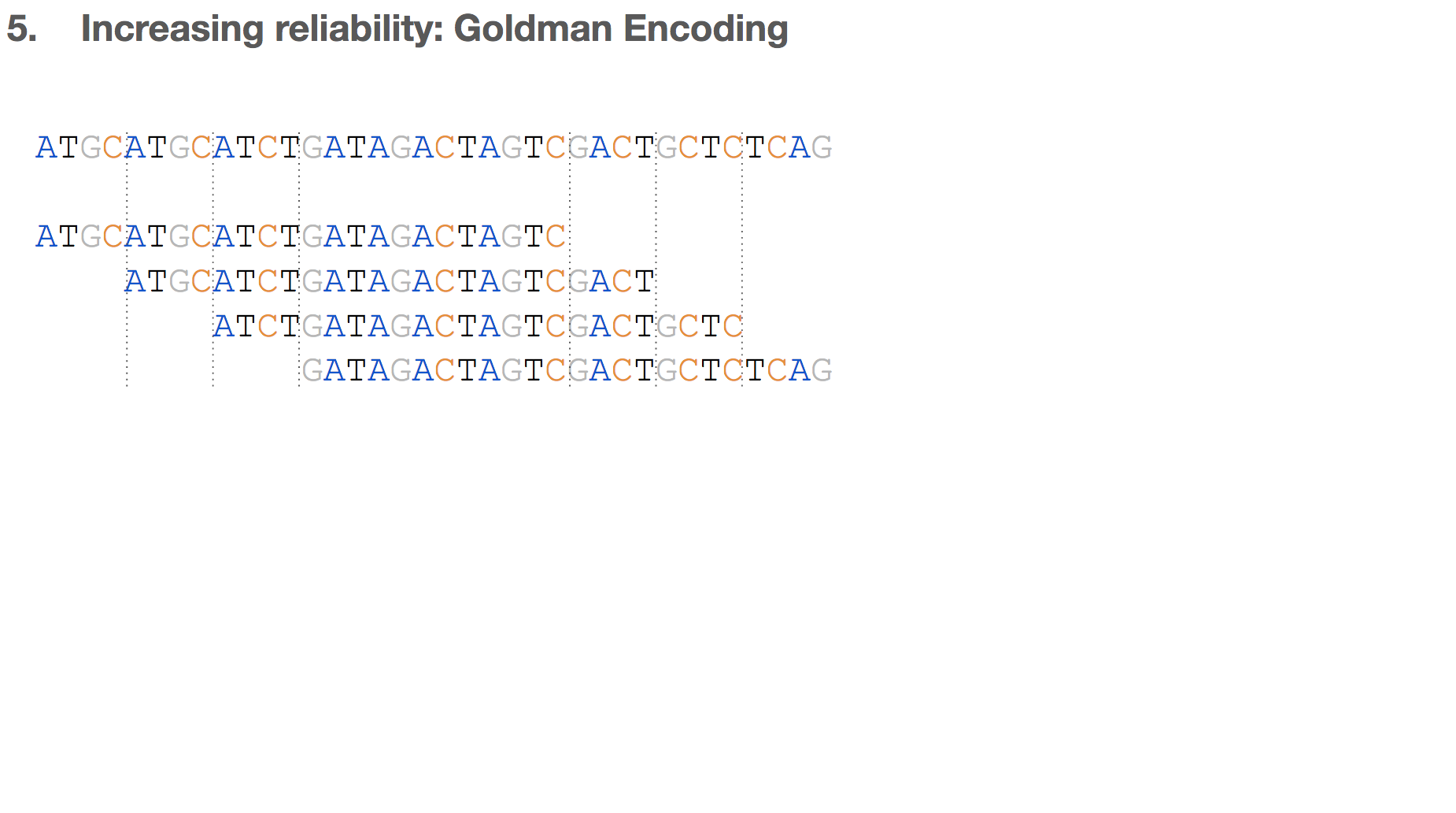
This is another example. Say we have some input nucleotides. We make many payloads that overlap with each other.
This creates many copies for a given nucleotide. For example, the C in the middle of the input nucleotides will be included in four different payloads. If one of them gets altered, it’s likely that three other copies will remain correct (because mistakes happen not that often) which will outnumber the mistake.
But, this only applies to the nucleotides in the body of the data. The head and tail of the data will be represented in much fewer copies, as little as one. This means that if there’s a mistake in the head or tail of the data, it’s unlikely that there will be other correct copies to rescue the mistake.
Another algorithm the researchers used for increasing reliability is XOR encoding which is commonly used in mathematics, electrical engineering, and computer science. While Goldman encoding was previously described, applying XOR algorithm for storing binary data in DNA was first described in this paper.
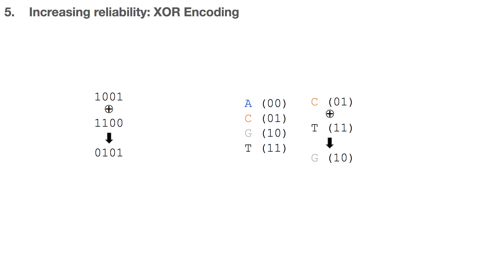
XOR means “exclusive or”. Given two inputs, the output is true only if the two inputs are different (or exclusive) from each other. This means that 1 XOR 0 is 1, but 1 XOR 1 is 0. We can apply this logic to DNA as well. For example if we say C is represented as 01 and T as represented in 11, C XOR T becomes G.
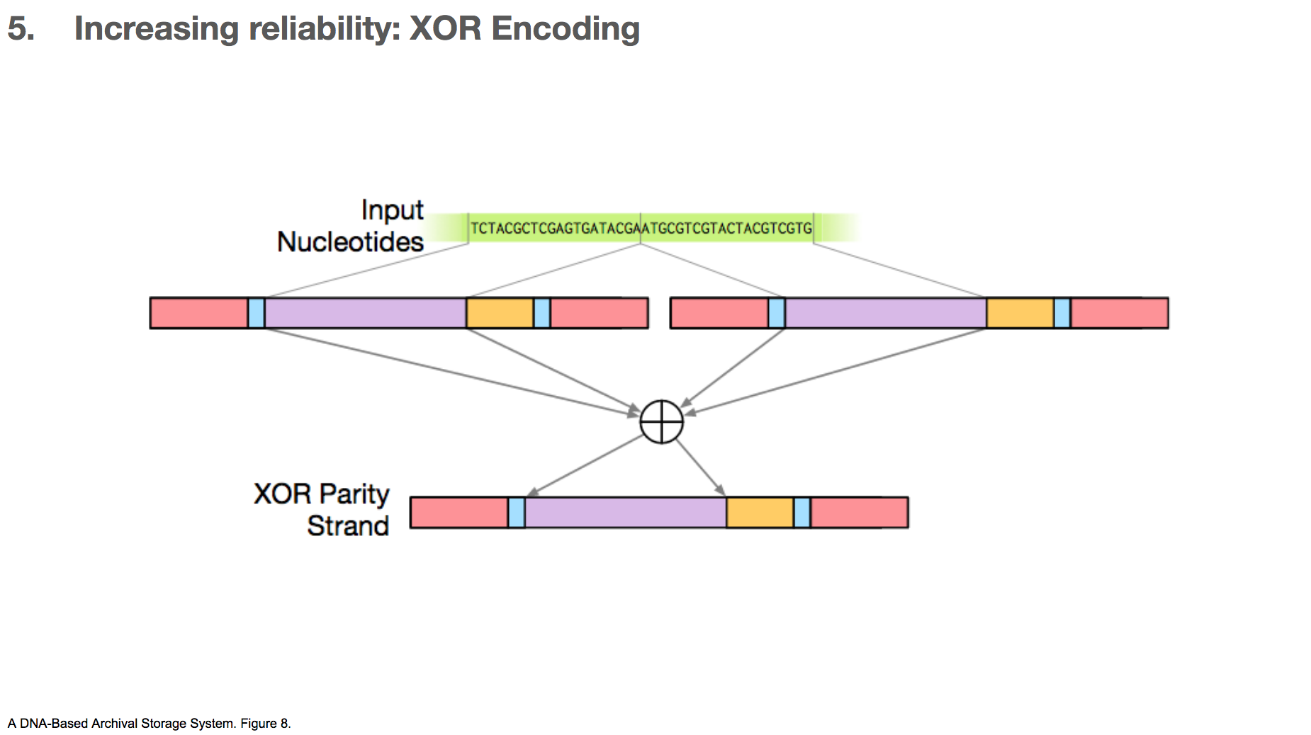
The researchers took two payloads, and XOR’d them to create a third payload.
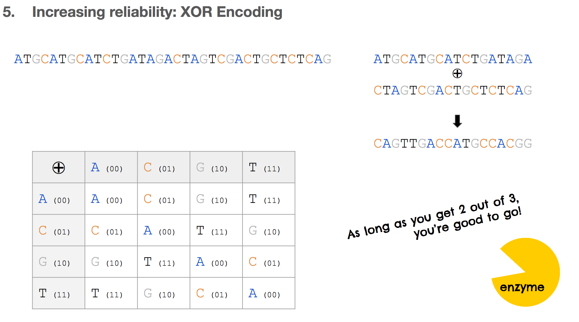
Let’s say we have some input nucleotides, and we came up with two payloads for that input nucleotides. We can create a third payload through XOR encoding. The table in the lower left shows the XOR of all possible pairs of nucleotides.
If there’s a mistake in one payload, as long as the other payload and the XOR payload are correct, we can correct the mistake.
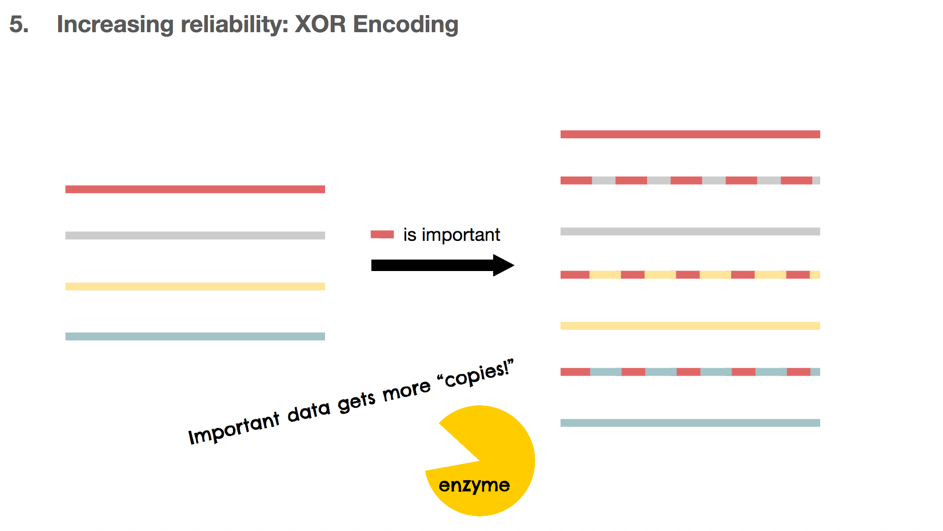
Another benefit of using XOR encoding is that we can make many copies for the important DNA piece. If the red DNA string is important, we can XOR the red one against the other DNA strings, creating three copies for the red DNA. These copies can also be used as copies for the other DNA strings, which means they’re multi-purpose.
In summary, the researchers transformed the original binary data into ternary data through Huffman encoding with a base of three. Then, they transformed the ternary data into DNA, avoiding repetition in nucleotides. To make sure there are additional copies that can correct mistakes, the researchers used either Goldman or XOR encodings.
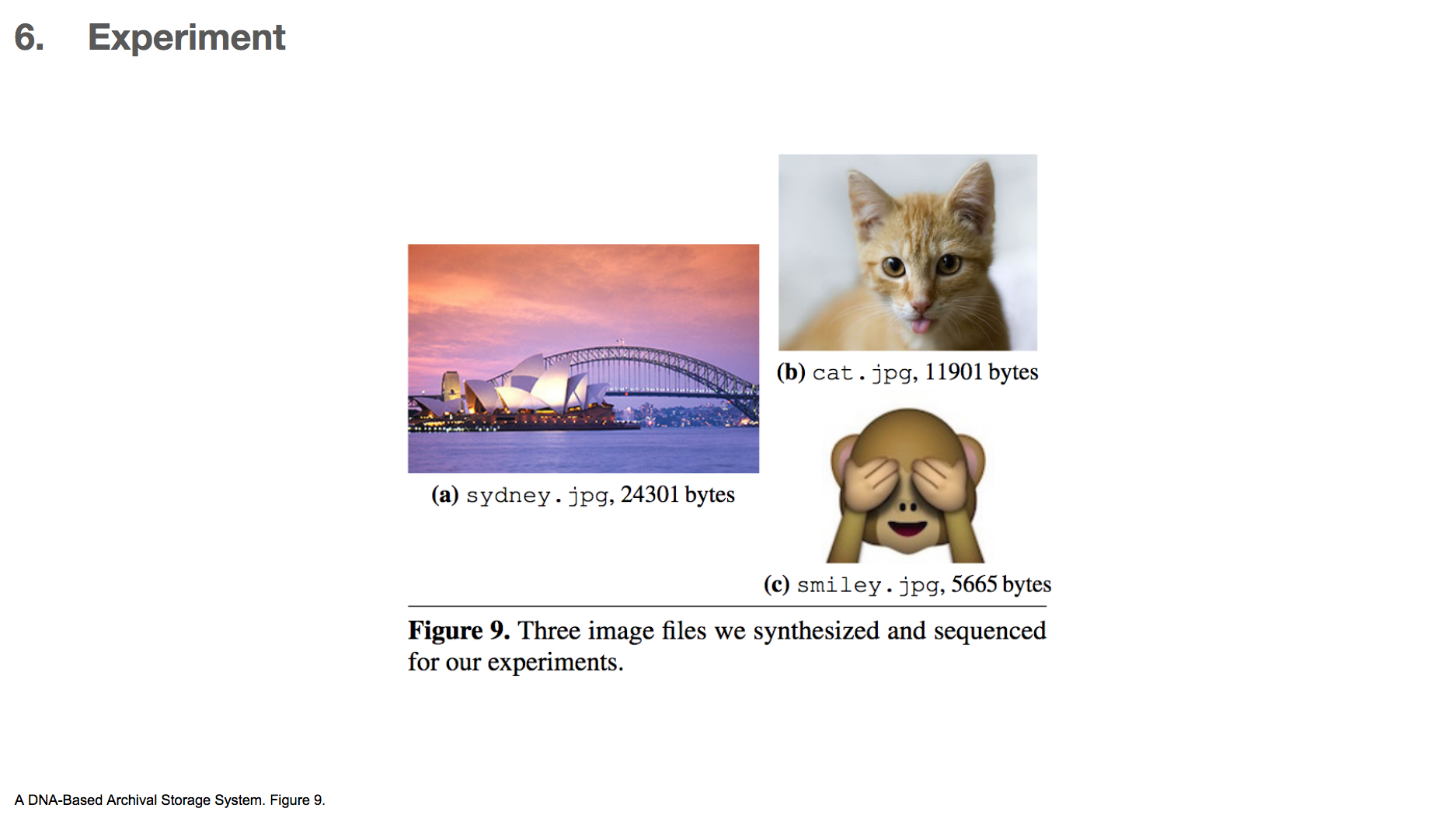
The researchers applied these algorithms to encode four different files, three of which were images and one of which was a text file. The three images files are shown above. The largest file they encoded was 24kB large, which is pretty small, but it was the largest anyone has ever encoded in DNA so far. To decode the DNA, they read the DNA strings and applied the algorithms backwards.
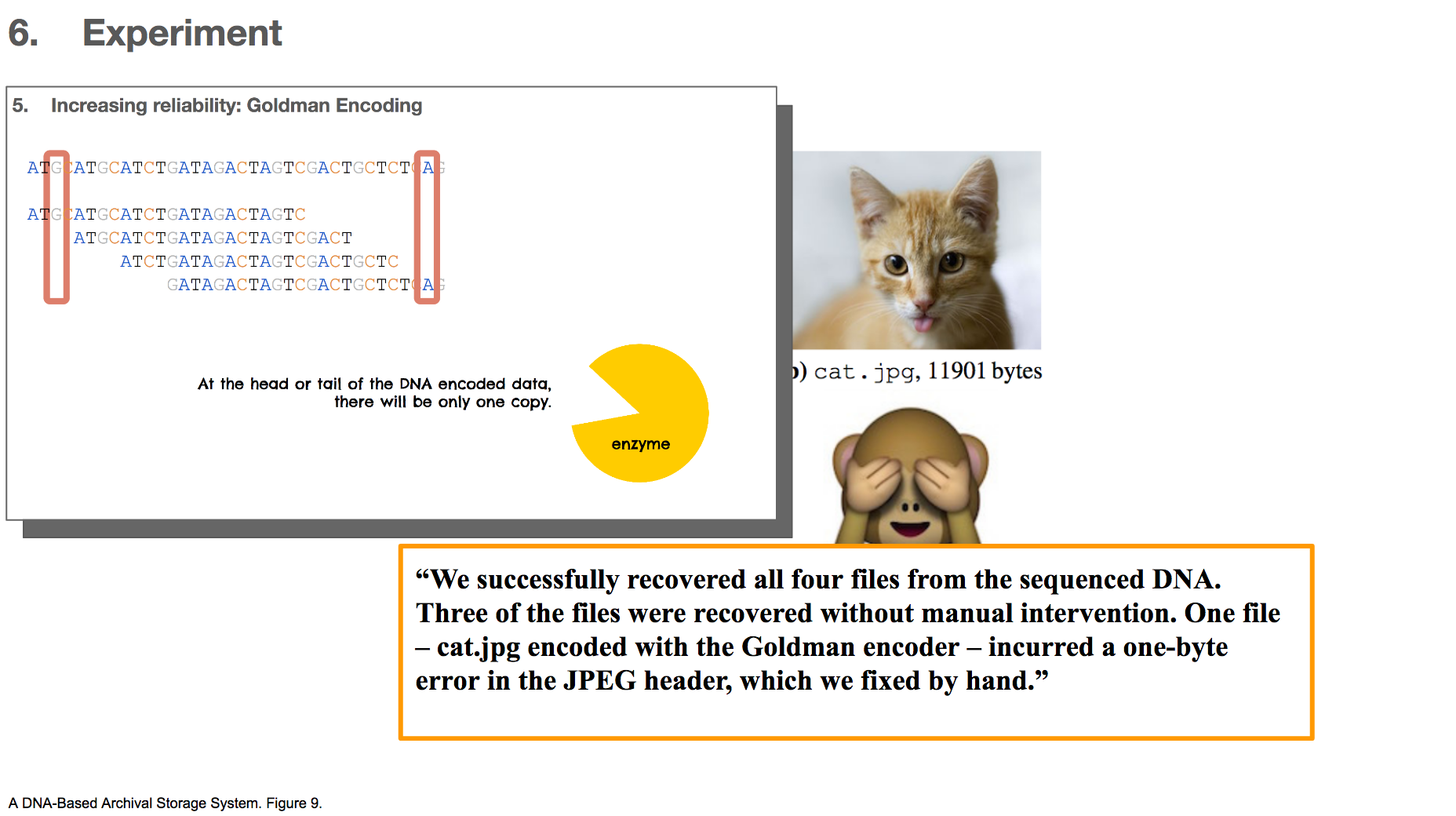
All encodings were successfully decoded without manual intervention, except for one – cat.jpg with Goldman encoding. There was a single byte error in the header of the file, which the researchers described as an easy fix. This error occurred probably because Goldman encoding does not make many copies of the head or tail of the data, and there probably wasn’t any correct copy (or very few) to rescue a mistake.
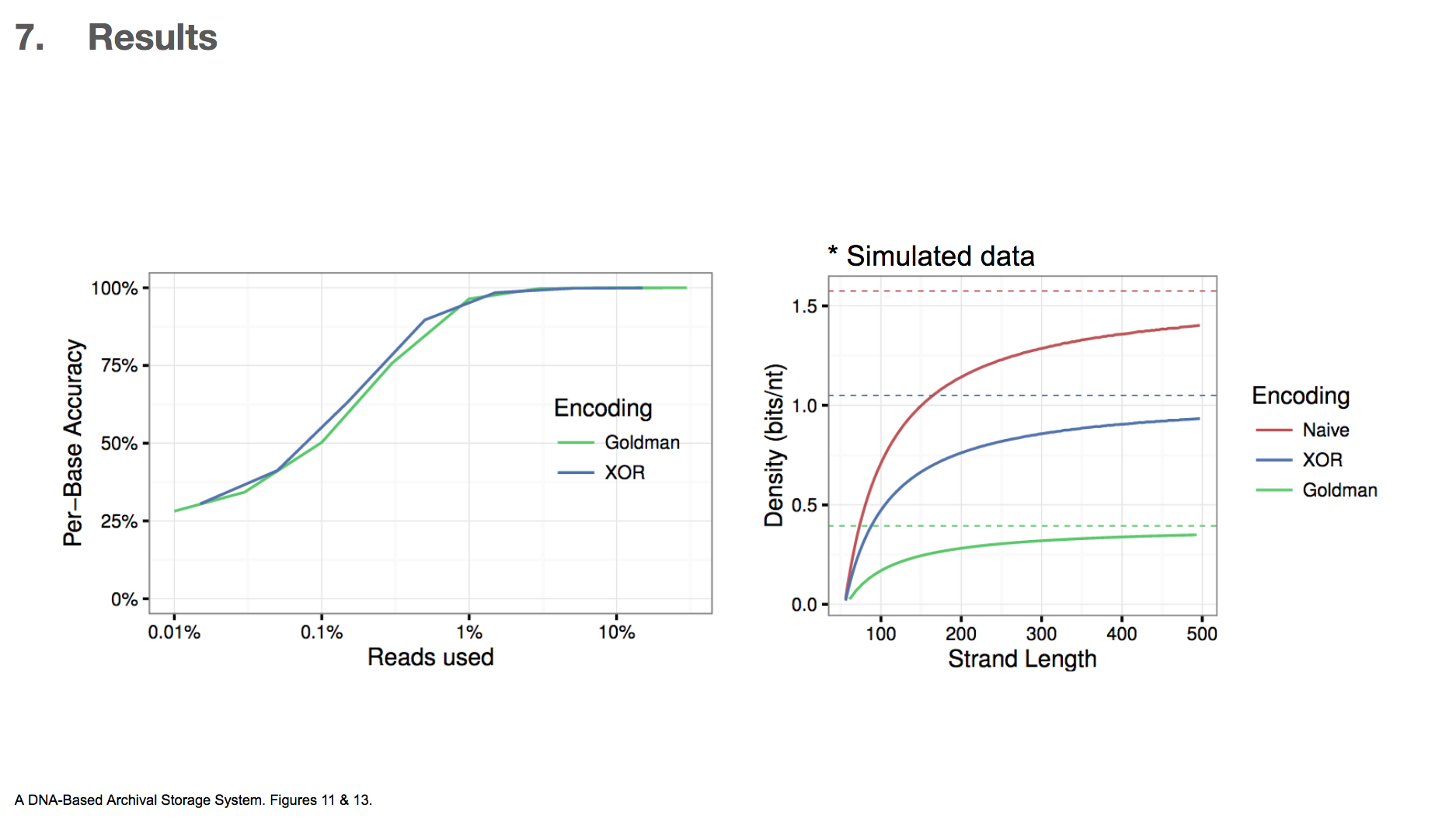
Because this was the first time XOR encoding was used in the context of DNA data storage, the researchers wanted to compare the efficiency between XOR and Goldman encodings.
The first graph shows data used vs. per-base accuracy. Reading DNA generates a lot of data, and the x-axis shows the fraction of the data that was actually used for decoding DNA. y-axis shows how accurate each base was, and therefore we want a graph that skews towards upperleft. This would mean that less data is sufficient for getting higher accuracy. They found that XOR encoding was slighly better than Goldman encoding in this criteria.
The second graph is based on simulated data, and it shows how much binary data can be encoded in DNA vs. DNA string length. In this paper, we’ve only seen DNA string length of 200 nucleotides. If we were to translate binary data directly to DNA by translating 00 into A, 01 into C and so on, then the density(bits/nt) will be 2. They found that XOR encoding can achieve higher density than Goldman encoding, which means less DNA is required to encode the same amount of binary data. The researchers concluded that this makes XOR encoding a more attractive option than Goldman encoding.
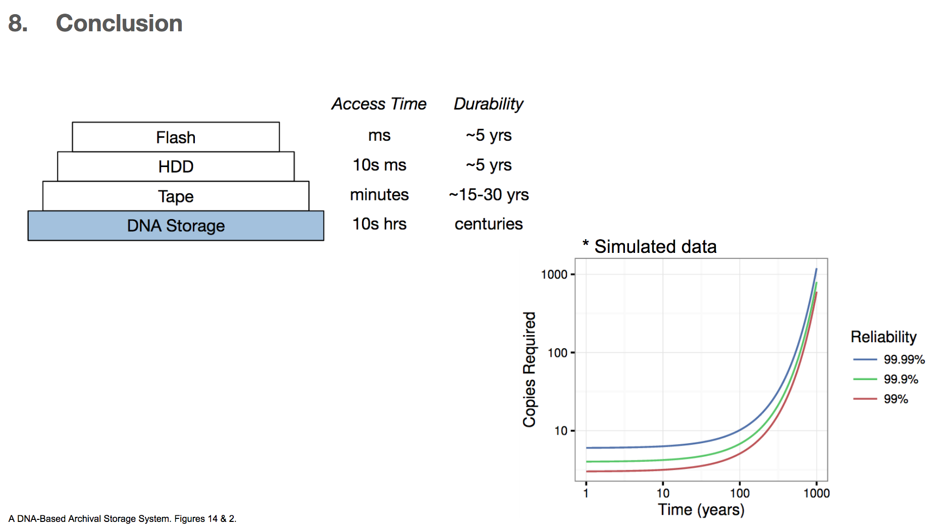
In conclusion, the researchers very much emphasize that this technology is for storing some data for a very very long time, and the data retrieval time is also very long compared to other existing technologies. They state that using DNA for storage system is best when we want to store data for centuries and can afford to have 10s of hours of retrieval time. For these reasons, we can imagine that storing important books is probably a good way to use this DNA archival storage system, but probably not storing a photo image of a pet that we want to see immediately when we want to see it.
The researchers also calculated the number of data copies required for a given length of storage time and the level of reliability wanted. DNA has a half life of 500 years, which roughly means that if we have two copies of DNA, one copy will degrade over the course of 500 years. They found that if we want 99.99% reliability and want to store the data for 100 years, then we only need 10 copies of the DNA encoded data. Given the high density of DNA (1 exabyte/1 mm³), storing ten copies will take up little space.
I hope you enjoyed learning something about biology, computer science, and the creative combination of both for a data storage system. I implemented the algorithm for transforming binary data into DNA in Rust, which you can learn more about here.
Thanks for reading!